Lab 02: Flexible Link Modeling
AE 443 · Experimental Dynamics and Control Laboratory · Spring 2026 · ERAU
Experiment Overview
Aircraft wings, helicopter rotor blades, and spacecraft solar panels are all flexible structures driven by servo actuators. Modeling them requires capturing not just the rigid-body motion of the actuator, but also the structural vibration modes of the flexible member attached to it. This lab derived the equations of motion for the SRV02 rotary flexible link system from first principles, experimentally identified the link’s stiffness from a free-oscillation test, and validated a 4-state state-space model against measured hardware responses.
- Derive the equations of motion for the servo-plus-flexible-link system using the Euler-Lagrange method
- Identify the link’s natural frequency ωn and rotational stiffness Ks from a free-oscillation decay experiment
- Build a 4-state state-space model (servo angle θ, link deflection α, and their derivatives)
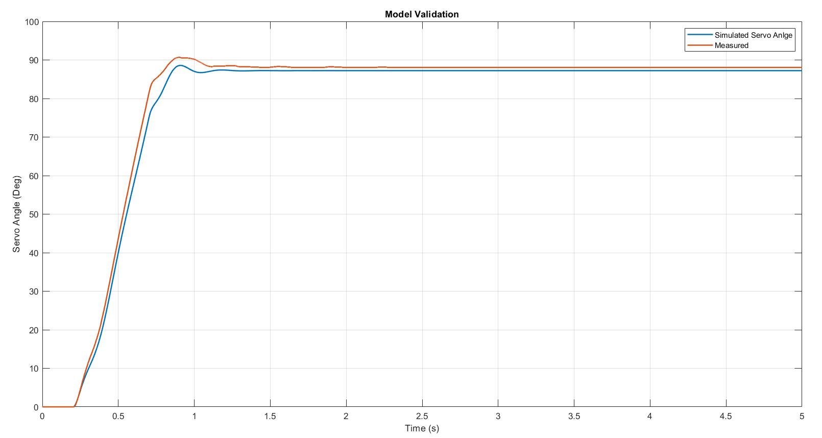
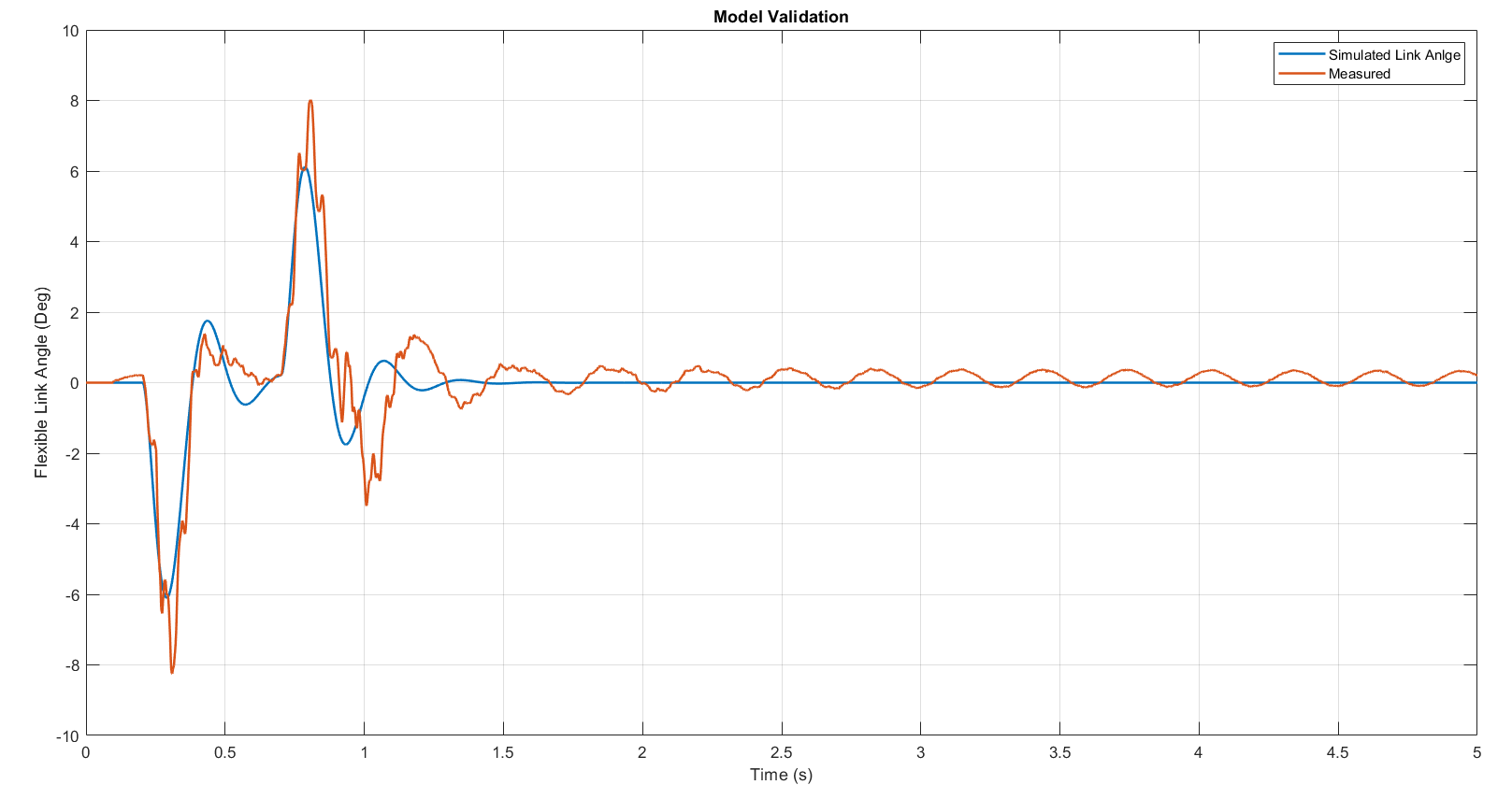
- Validate the model by comparing simulated and measured responses to a step motor command
Equipment & Tools
- Quanser SRV02 rotary flexible link system (ml = 0.065 kg, Ll = 0.419 m)
- Strain gauge sensor embedded in the flexible link for deflection angle measurement
- Q2-USB data acquisition board
- VoltPAQ power amplifier
- MATLAB/Simulink with QUARC real-time toolbox (setup_flexgage.m and q_flexgage_val model)
Approach & Equations of Motion
The system Lagrangian L = T − V was formed using the kinetic energy of both the servo base and the flexible link, and the elastic potential energy stored in the link spring. Applying the Euler-Lagrange equations to each generalized coordinate produced coupled second-order differential equations. These were rewritten in first-order state-space form ẋ = Ax + Bu, with states x = [θ, α, θ̇, α̇].
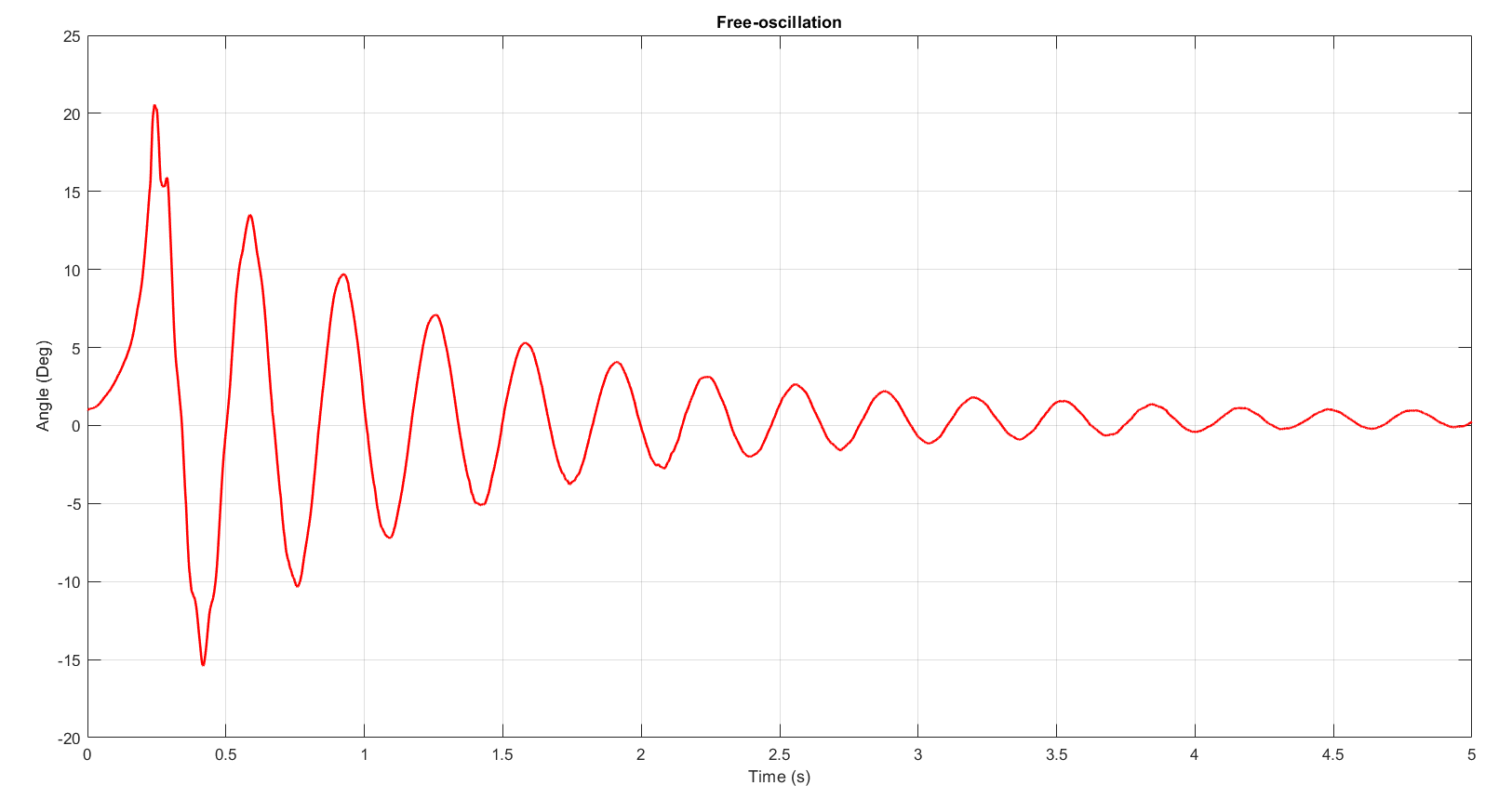
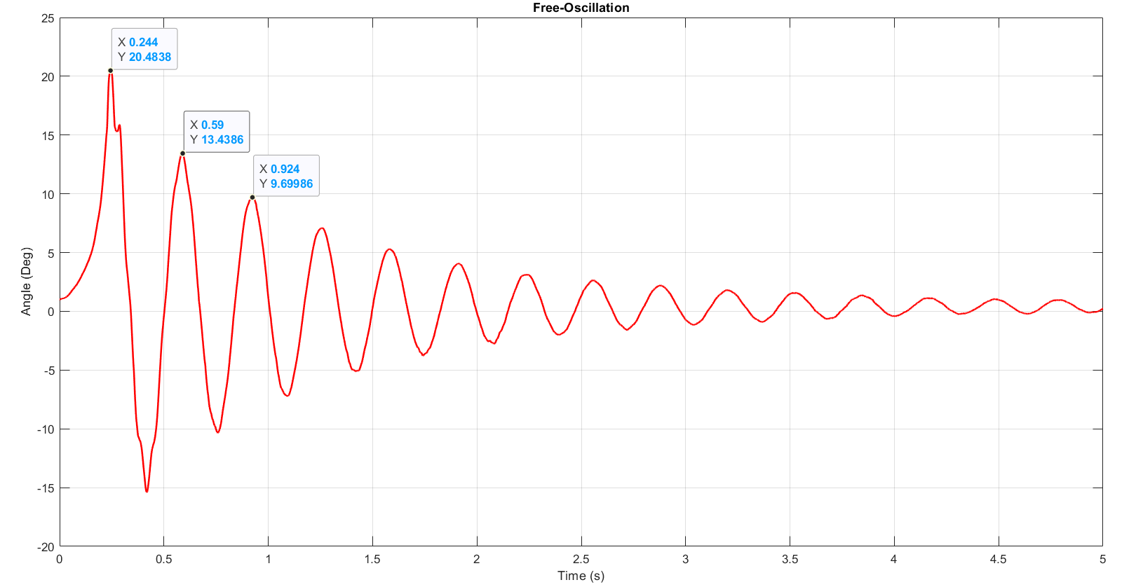
Link stiffness was determined experimentally by freely oscillating the link with the servo locked, measuring successive peak amplitudes to compute the damped natural frequency ωd and damping ratio ζ, then recovering the undamped natural frequency and applying:
Ks = Jl · ωn² where Jl = mlLl² / 3
Key Results
- From peak amplitudes O1 = 20.48° at t = 0.244 s and O3 = 9.70° at t = 0.924 s: Tosc = 0.34 s, ωd = 18.48 rad/s, ζ = 0.034.
- ωn = 18.49 rad/s and Ks = 1.30 N·m/rad.
- Open-loop poles: P1 = 0 (marginally stable); P2,3 = −8.16 ± 22.52i (stable oscillatory modes); P4 = −24.01 (stable).
- The pole at the origin indicates the system is marginally stable in open loop: a constant motor input causes the servo angle to drift without bound, while the flexible link oscillates at ~22.5 rad/s before damping out.
- Simulated and measured servo angle responses agreed closely in rise time and steady state. The flexible link angle matched the correct oscillation frequency but showed slight amplitude discrepancy from unmodeled structural damping.
MATLAB Code
Three scripts handled the free-oscillation plot, model validation comparisons, and state-space to transfer function conversion.
% Free-oscillation plot
plot(data_alpha(:,1), data_alpha(:,2), 'r', 'LineWidth', 1.5);
xlabel('Time (s)');  ylabel('Angle (Deg)');  title('Free-Oscillation');

% Model validation – servo angle overlay
plot(data_theta(:,1), data_theta(:,2), 'LineWidth', 1.5);  % simulated
hold on
plot(data_theta(:,1), data_theta(:,3), 'LineWidth', 1.5);  % measured
legend('Simulated Servo Angle', 'Measured')

% State-space ? transfer function and open-loop poles
sys   = ss(A, B, C, D);
TF    = tf(sys);         % 2×1: [theta(s)/u(s); alpha(s)/u(s)]
poles = eig(A)           % P1=0, P2,3=-8.16±22.52i, P4=-24.01
Valuable Takeaways
- A marginally stable open-loop system requires feedback control. The pole at the origin means the servo drifts without constraint, directly motivating why real flexible-link systems — like aircraft control surfaces and robotic manipulators — use closed-loop control rather than open-loop commands.
- Structural stiffness can be identified from a simple free-oscillation test. Measuring three successive peak amplitudes and applying the logarithmic decrement method extracted Ks from experimental data alone — no physical material test required.
- State-space models connect physics to control design. The A matrix derived from the Euler-Lagrange equations is the same matrix whose eigenvalues define stability, whose structure determines observability and controllability, and whose entries feed directly into LQR or pole-placement controller designs.
- Gained hands-on experience connecting Lagrangian mechanics, linear system theory, and real hardware validation — the full workflow from equation derivation to experimental confirmation used in aerospace structural dynamics and flexible-body control research.